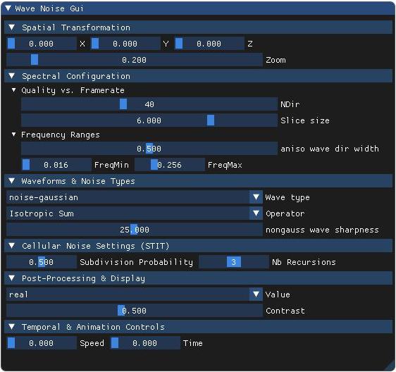
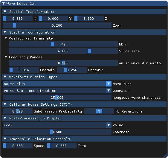
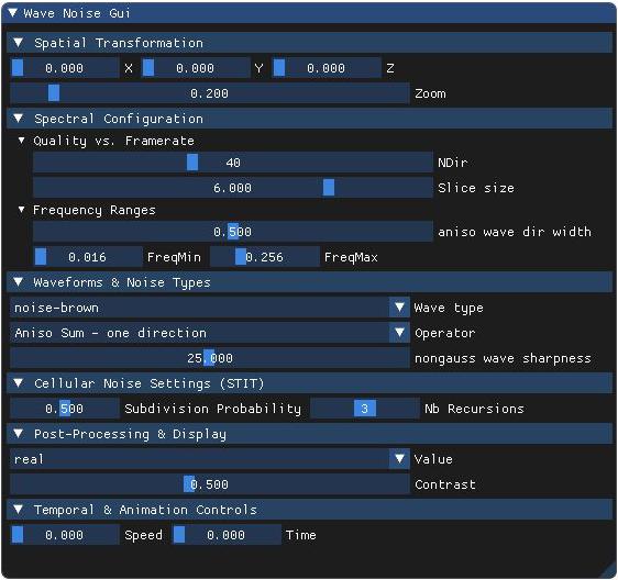
Wave Noise GUI
Jump to section:
- 🧭 Spatial Transformation
- 📈 Spectral Configuration
- 🔬 Waveforms & Noise Types
- 🧩 Cellular Noise Settings (STIT)
- 🎛️ Post-Processing & Display
- ⏱️ Temporal & Animation Controls
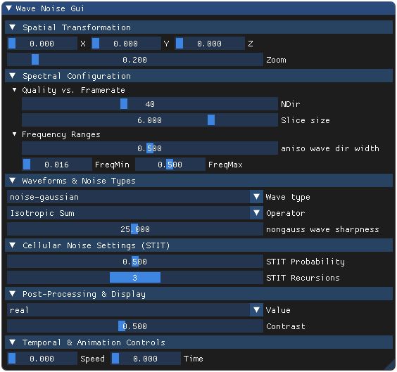
🧭 Spatial Transformation
These parameters control the spatial placement and scale of the noise in 3D space. They allow translating the noise field and adjusting its frequency globally. Useful for positioning, tiling, or zooming into specific structures.
Controls the position and spatial scale of the noise in 3D space. These parameters define how the noise field is placed, zoomed, or panned, similar to camera controls for textures.
- X, Y, Z – Translates the noise field along each axis
- Zoom – Scales the noise frequency globally (higher zoom = denser pattern)
- X
- Translation offset along the X axis, used to move the noise pattern horizontally in space.
- Y
- Translation offset along the Y axis, used to move the noise pattern vertically in space.
- Z
- Translation offset along the Z axis, allowing to explore noise variations in depth or animation.
- Zoom
- Scales the input position vector before evaluating the noise. Increasing the zoom makes the noise pattern appear smaller and more detailed.


📈 Spectral Configuration
These parameters define how the frequency domain is sampled and how directions are distributed. They influence the resolution, angular diversity, and frequency bandwidth of the generated waves.
Defines how the spectral domain is sampled and how directional and frequency resolution is distributed. These parameters are now grouped by function: some control visual quality and performance, others define the actual frequency content.
Quality vs. Framerate
- Slice size (RATIO) – Controls the spectral sampling resolution. Lower values improve precision but increase alignment; higher values reduce quality but speed up rendering.
- NDir – Number of angular directions used in wave synthesis. More directions produce smoother noise at a higher computational cost.
Frequency Ranges
- Aniso wave dir width – Angular spread used in anisotropic sampling. Controls the angular domain of wave propagation.
- FreqMin – Lower frequency bound. Eliminates large-scale components below this threshold.
- FreqMax – Upper frequency bound. Removes fine details beyond this threshold.
- Slice size
-
Controls the spatial frequency of the wave noise by scaling the distance between successive wavefronts.
Internally, this parameter is converted to a frequency ratioRATIO = 2iRatio, which is used to scale the wave pattern in the shader.- Low slice size → low frequency (large features)
- High slice size → high frequency (small details)
1.0 / RATIOin the phase computation of each wave.
Use this to zoom into or out of the structural level of the noise without changing the global zoom factor. - NDir
-
Number of wave directions used to sample the spectral domain.
This controls how many hyperplanar waves are superposed to construct the final noise.- Low values (e.g. 8–16) → faster computation, coarser noise with more visible repetition or banding.
- High values (e.g. 64–100) → smoother, more isotropic noise but with higher computation cost.
Operator(e.g., isotropic vs anisotropic).
This parameter balances quality and performance. It affects both the spatial frequency content and the angular regularity of the noise field. - Aniso wave dir width
-
Controls the angular spread of directions used in anisotropic wave noise modes.
A smaller value restricts the wave sampling to a narrower set of directions, producing strongly oriented patterns (e.g., flow lines, fibers). A higher value allows for more angular diversity, resulting in a more diffuse anisotropy.
This parameter modulates the spread of the angular sector used in the wave sampling stage, especially inOperatormodes 1 and 2. - FreqMin
-
Sets the lower bound of the frequency band used to generate the wave noise.
Frequencies below this threshold are filtered out and do not contribute to the noise.
IncreasingFreqMinremoves large-scale structures, making the noise more fine-grained. - FreqMax
-
Sets the upper bound of the frequency band used in wave generation.
Frequencies above this value are discarded. LoweringFreqMaxsmooths out small-scale details.
Together,FreqMinandFreqMaxdefine a band-pass filter in the spectral domain.


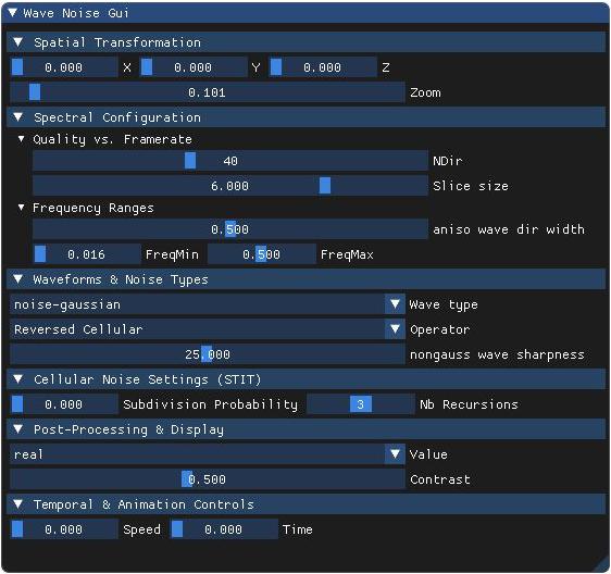
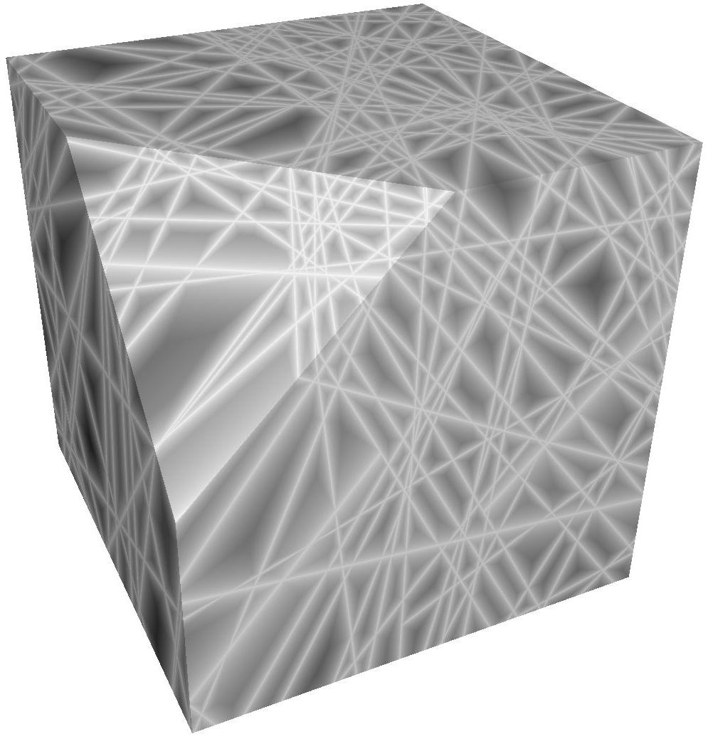
🔬 Waveforms & Noise Types
These parameters determine the waveform shapes and the synthesis strategy used to create the noise. They control the spectral shape (Gaussian, non-Gaussian, etc.) and the model used (e.g., isotropic, cellular).
Controls the shape and combination of waveforms used to generate noise. This includes spectrum shaping (Gaussian, non-Gaussian) and the synthesis strategy (sum, cellular, etc.).
- Wave type – Defines the spectral profile (e.g., Gaussian, marble, crystal)
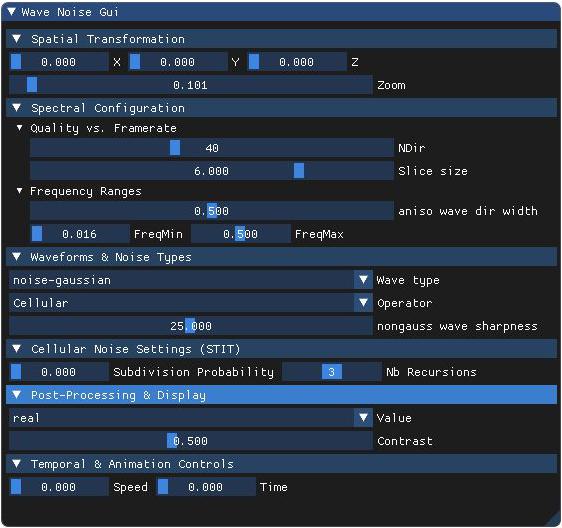
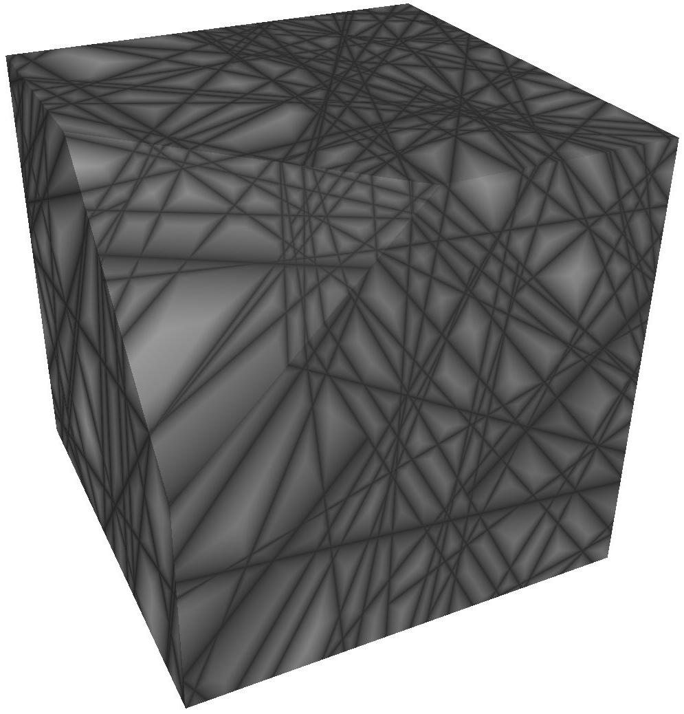
- Operator – Chooses the synthesis model (e.g., isotropic sum, STIT)
- Non-gauss wave sharpness – Sharpness of non-Gaussian wave profiles
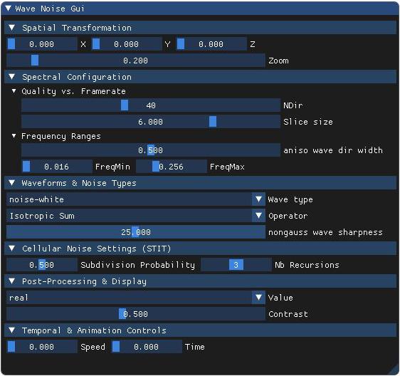
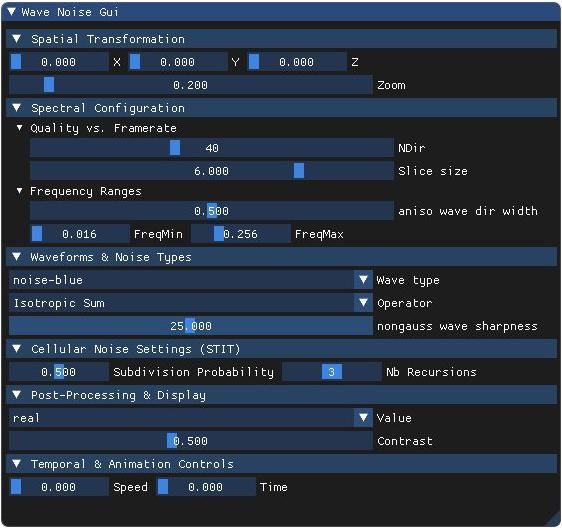
- Wave type
-
Selects the base amplitude profile used to construct the procedural wave noise. Each mode defines a different spectral distribution or structural appearance:
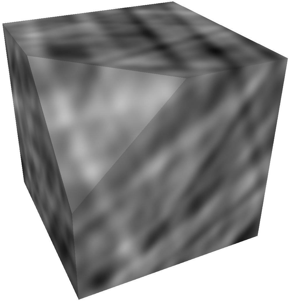
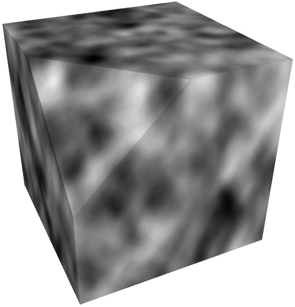
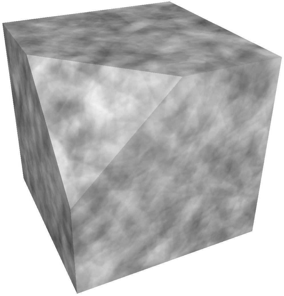
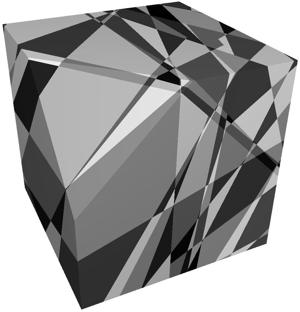
- 0 – noise-gaussian : Gaussian frequency falloff — smooth, bell-like spectrum. Ideal for natural, soft noise.
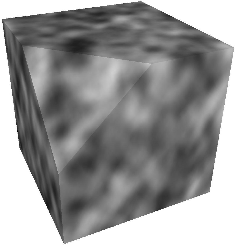
- 1 – noise-white : Uniform amplitude spectrum — high entropy, fully uncorrelated noise.
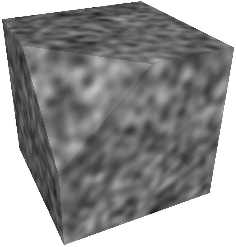
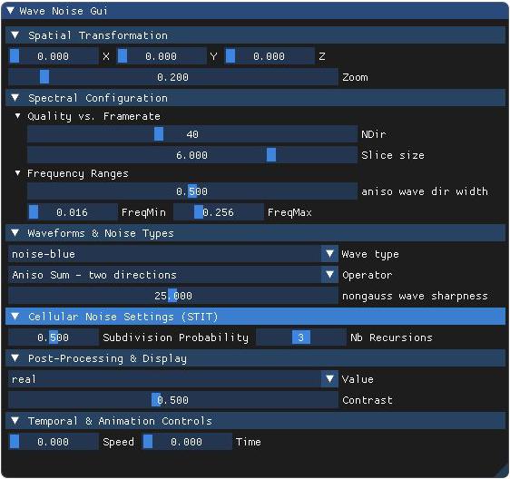
- 2 – noise-blue : Increasing amplitude with frequency — enhances fine details and sharp transitions.
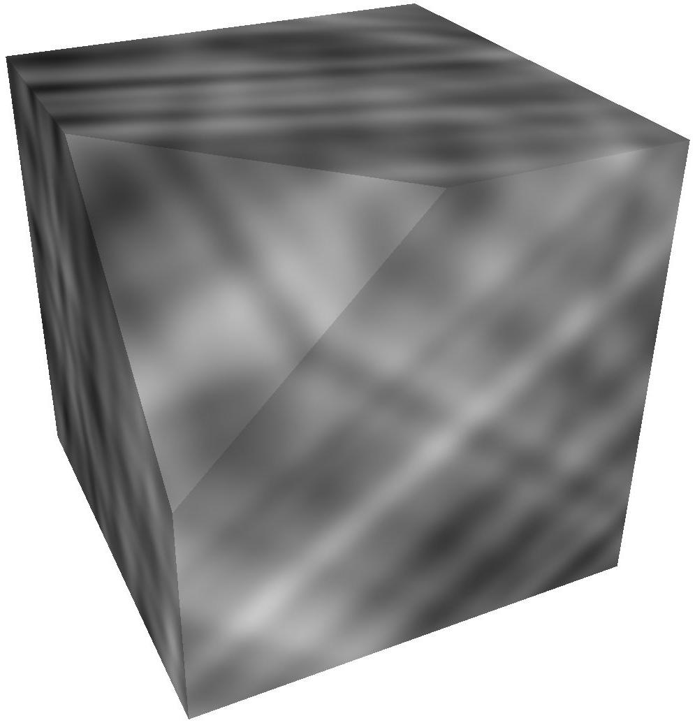
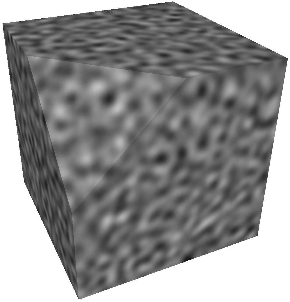
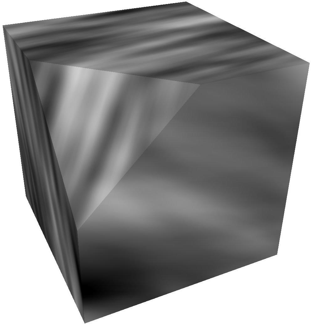
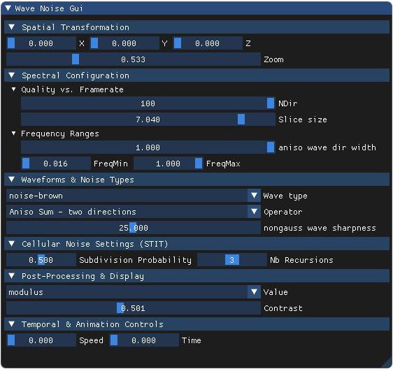
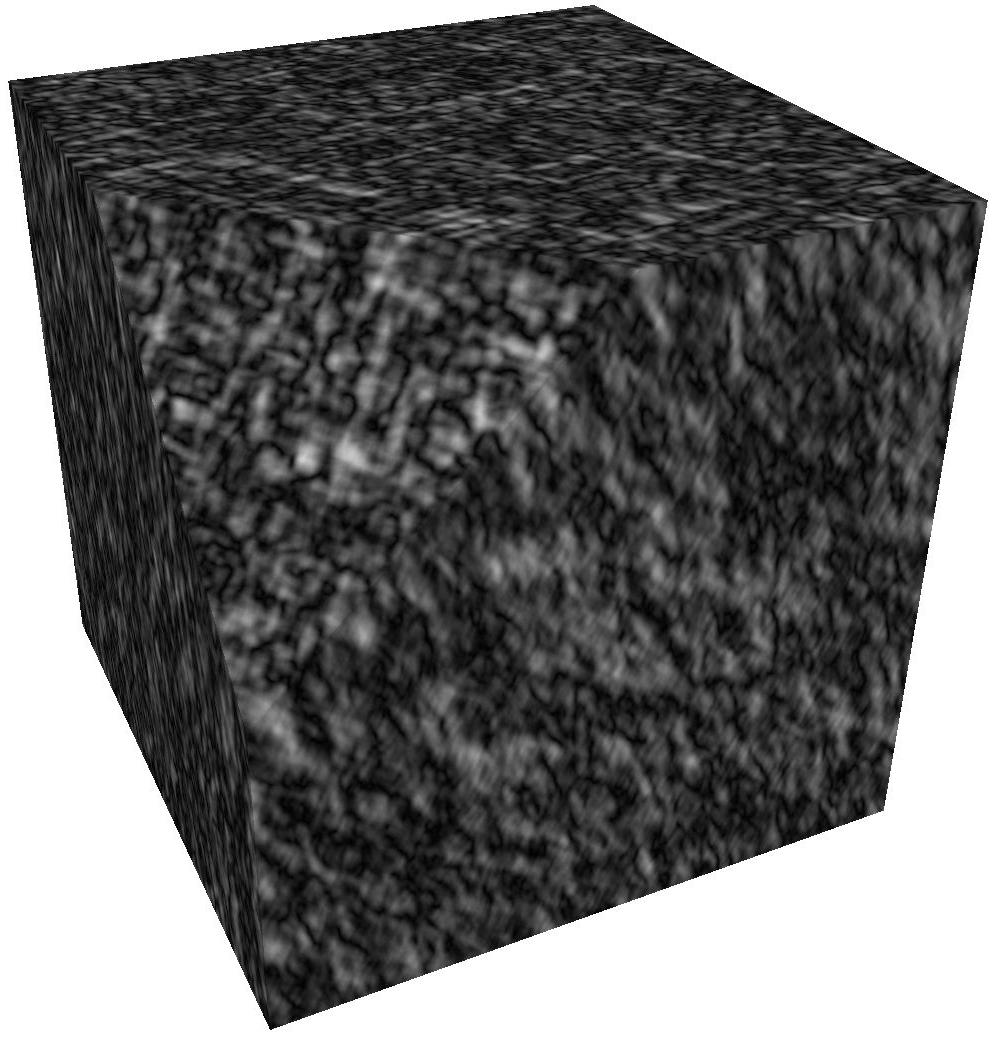
- 3 – noise-brown : Dominated by low frequencies — produces large-scale cloudy variations.
- 4 – nongauss-crystal1 : Sharp symmetric peaks — mimics crystalline or polygonal features using a periodic non-Gaussian waveform.
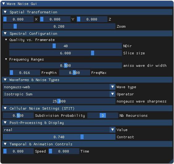
- 5 – nongauss-web : Composed of many narrow peaks — creates thread-like structures and sparse interference.
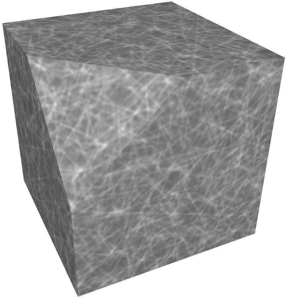
- 6 – nongauss-marble : Based on triangular or stair-stepped waveforms — results in periodic veining patterns like marble.
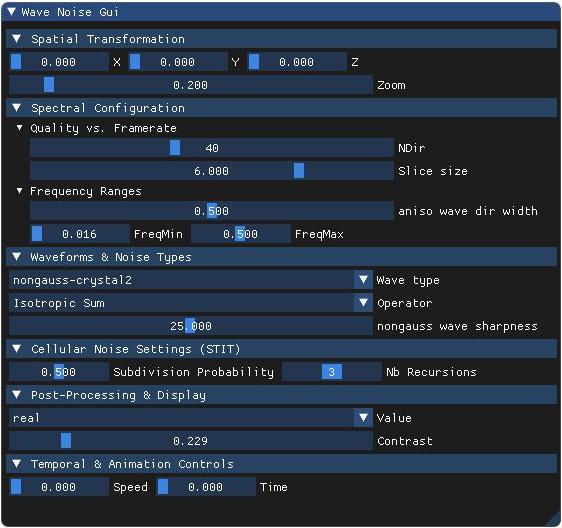
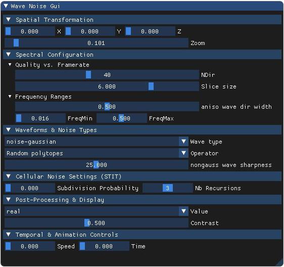
- 7 – nongauss-crystal2 : Multi-step waveform — alternative symmetry to crystal1, using flat intervals and hard transitions.
- 8 – nongauss-scratches : Thresholded Fourier noise — results in scratch-like elongated segments with directional bias.
- 9 – nongauss-smooth cells : Soft, cell-based structure using normalized power spectrum and non-linear modulation.
- 10 – noise-two ampli levels : Two distinct amplitude levels — inspired by STIT patterns, generating layered contrast bands.
Contrast,Speed, andTime. It also interacts with the rendering mode controlled by theOperator. - Operator
-
Selects the noise generation strategy, corresponding to different classes of procedural models:
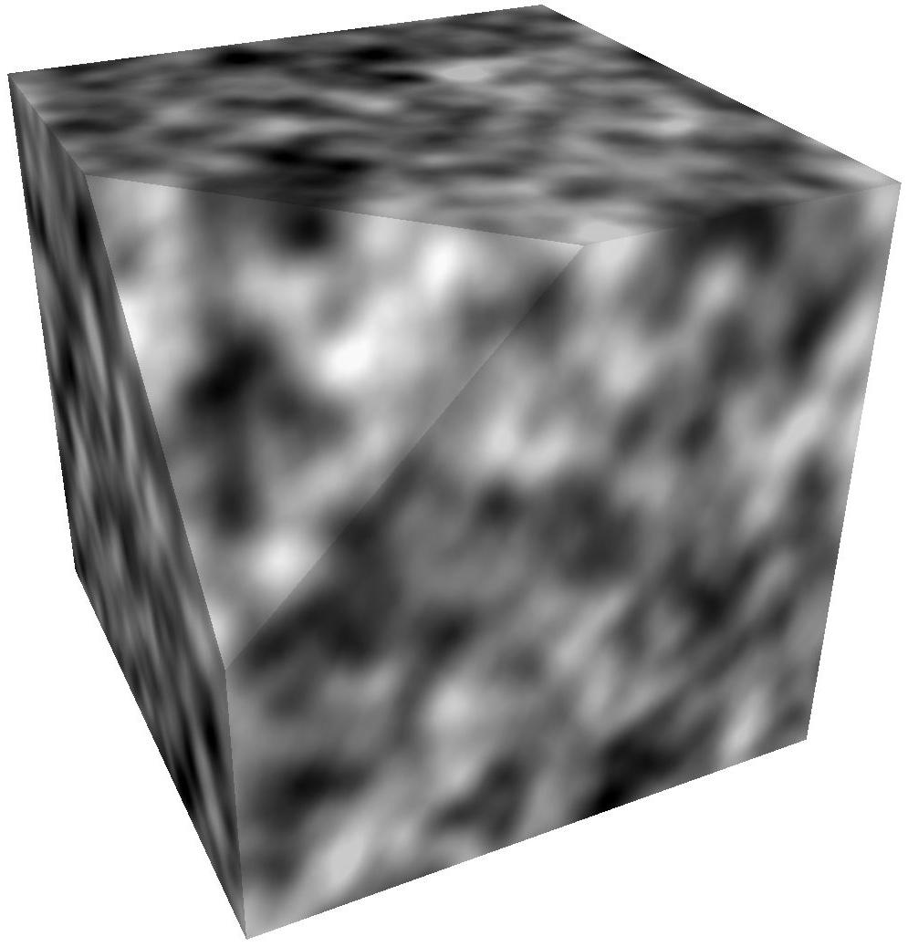
- 0 – Isotropic Sum: Uses a superposition of isotropic wave functions in random directions. The noise is fully directional-uniform, suited for general-purpose use.
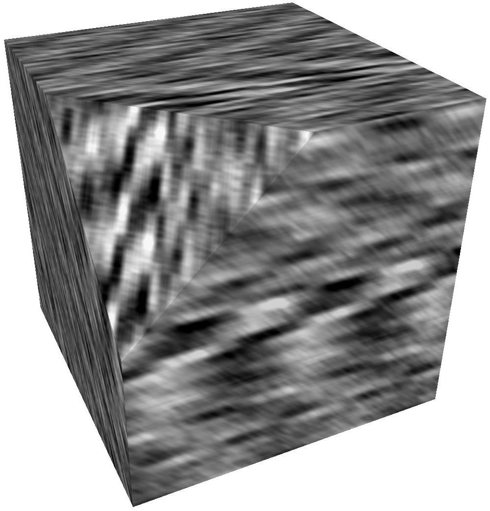
- 1 – Aniso Sum: Uses anisotropic wave sampling in one set of preferred directions. Produces directional structures and oriented features.
- 2 – Two Aniso: Combines two distinct sets of anisotropic orientations. This increases directional richness while preserving anisotropy.
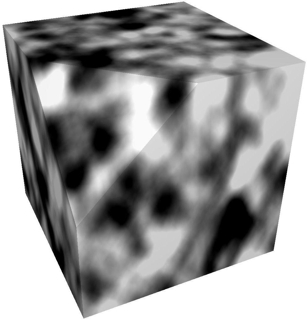
- 3 – Simple STIT: Applies a recursive cell subdivision using distance thresholds on the wave function. Generates structured cellular patterns with a uniform recursive rule.
- 4 – STIT Nonlinear: Adds non-linearity through a power function and contrast amplification. Results in more stylized, high-contrast cellular noise.
- 5 – STIT Step: Produces binary-like segmented noise using a step function. Good for thresholded structures such as scratches or material discontinuities.
- 6 – STIT Inverse: Applies an inverse exponential mapping on the wave result. Enhances boundaries and voids, creating inverted cellular contrast.
Contrast,NRec(recursion depth), andProba(split probability). - Non-gauss wave sharpness
-
Adjusts the shape of non-Gaussian wave profiles by modifying their sharpness or steepness.
This parameter influences how rapidly the wave function rises and falls. Low values yield smoother, softer profiles; high values generate sharper peaks or edges.
It is primarily used in non-Gaussian wave types (e.g., crystal, marble, web), and affects both frequency content and visual appearance.
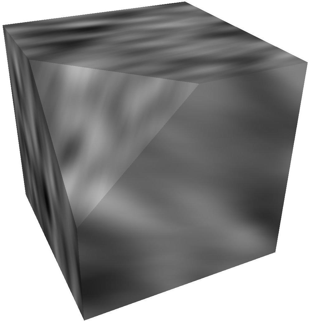
Isotropic Gaussian noises:
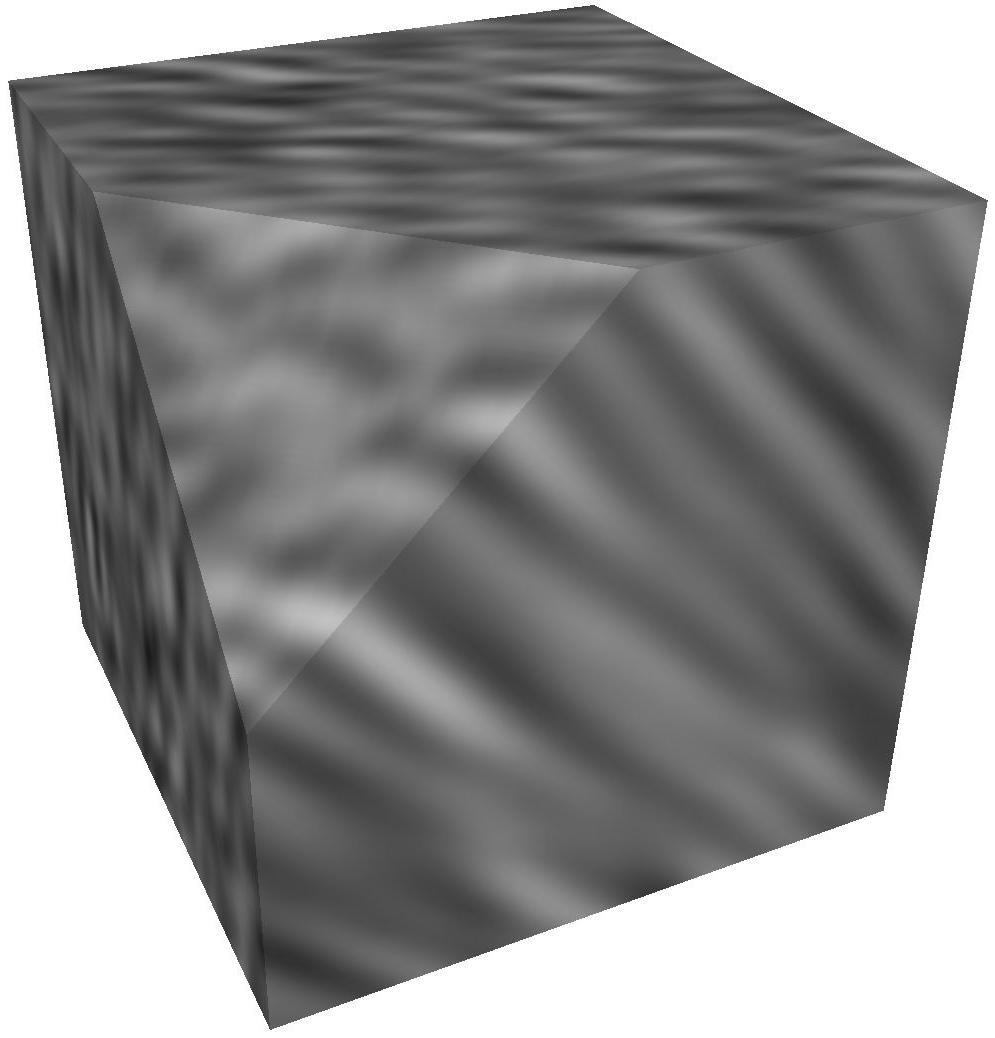
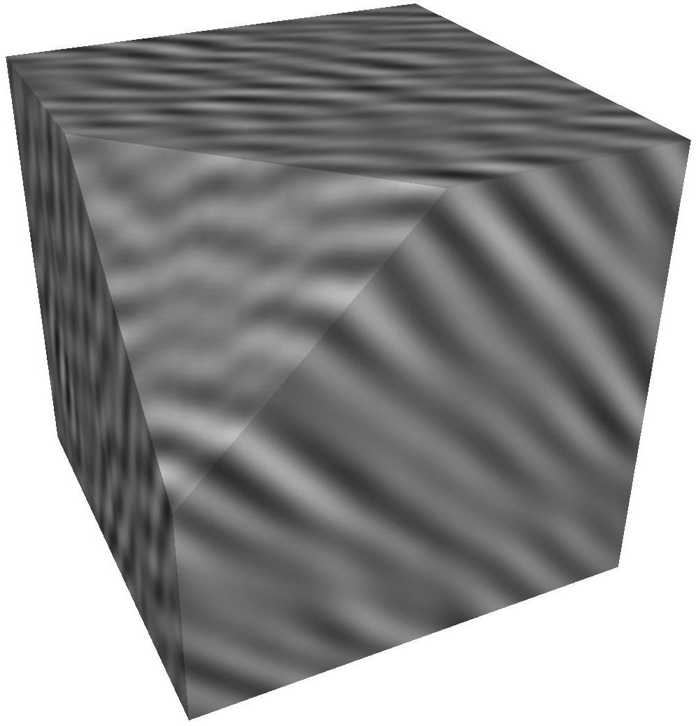
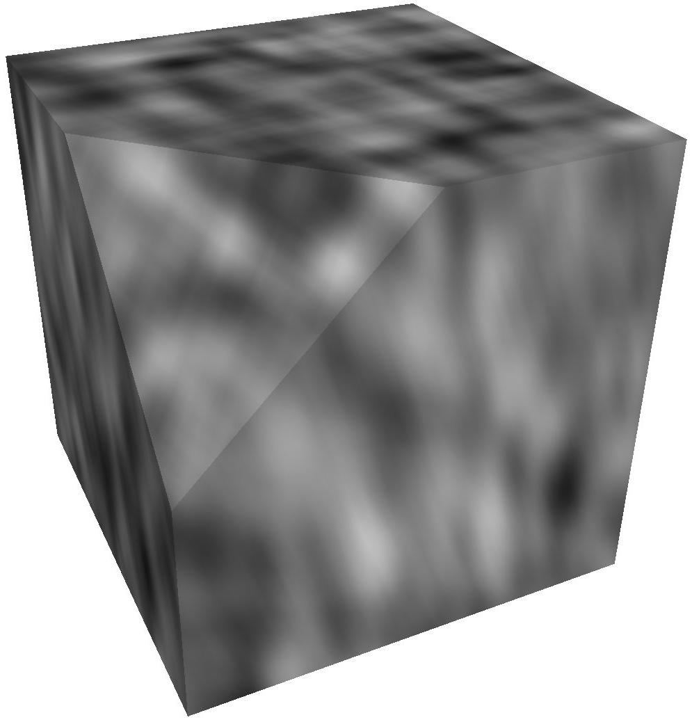
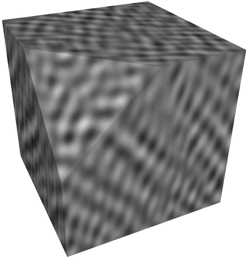
Anisotropic Gaussian noises (1 direction):

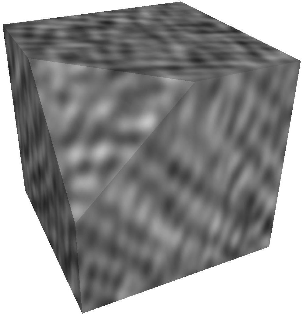
Anisotropic Gaussian noises (2 directions):


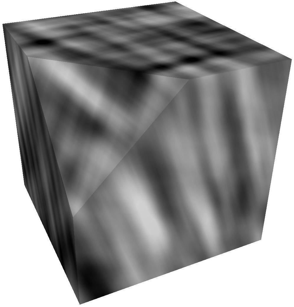
Non-Gaussian noises:

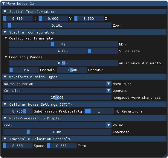
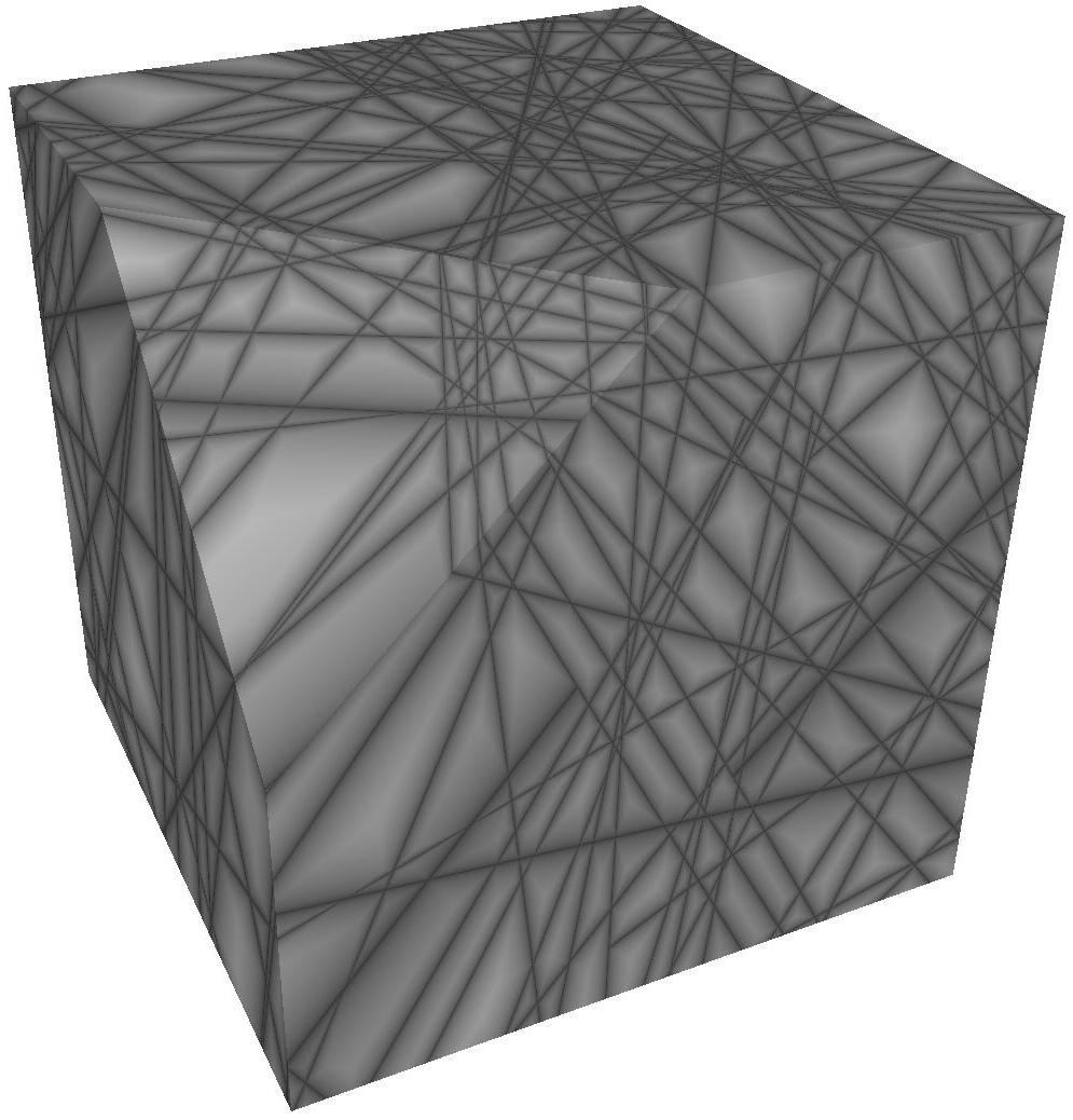
🧩 Cellular Noise Settings (STIT)
Specific to recursive cellular models (STIT), these settings control how and when cells split. They influence the level of detail, variability, and complexity in cell-based noise patterns.
Used in recursive cell-based operators (STIT). These values define how many splits occur and how likely each split is, controlling structure complexity and detail.
- STIT Probability – Probability of cell subdivision at each recursive level
- STIT Recursions – Maximum number of recursive subdivisions
- STIT Probability
-
Controls the probability of recursively splitting a cell during wave-based STIT (Stochastic Iterative Tessellation) generation.
At each recursion step, a random value is drawn and compared to this probability:
If the draw is belowSTIT Probability, the cell is split again using a new wave; otherwise, recursion stops.
- Low values (e.g. 0.2) → most cells are split once or twice → large, simple cells.
- High values (e.g. 0.9) → many recursive splits → smaller, more complex cellular patterns.
Operatormodes 3 to 6. - STIT Recursions
-
Specifies the maximum number of recursive cell splits allowed in STIT-based noise models.
Each recursive level adds more detail and subdivisions to the cell structure, up to the number defined bySTIT Recursions.
- 1–2 recursions → coarse patterns with few internal boundaries.
- 4–6 recursions → rich, intricate cell structures with fine details.
STIT Probability, it governs both the depth and randomness of cell subdivision in recursive operators.
🎛️ Post-Processing & Display
These parameters are applied after the core noise generation to adjust its visual appearance. They affect contrast, interpretation of complex noise values, and how scalar values are extracted for rendering.
Affects how the complex noise result is converted to scalar values and visualized. These controls tune contrast and select which component of the noise is shown.
- Contrast – Amplifies or flattens the differences in the noise output
- Value (QQ) – Chooses how the complex noise is interpreted (real, phase, magnitude...)
- Contrast
-
Adjusts the visual contrast of the noise pattern without altering its structure.
This multiplier scales the amplitude of the wave noise before display. A value of0results in a flat mid-gray image, while1preserves the full dynamic range of the noise.
It helps reveal fine structures and can improve visual readability, especially when visualizing small variations or comparing multiple patterns.Note: the behavior of the
Contrastparameter depends on the selectedOperator:-
Operators 0–2 (wave-based noise): contrast is applied as a simple linear scaling:
val = clamp(contrast × waven.x + 0.5, 0.0, 1.0)
This directly adjusts the amplitude of the wave signal around a central base level. -
Operators 4 and 6 (non-Gaussian / cellular wave models): contrast is applied as a non-linear exponent:
val = pow(clamp(...), contrast)
This amplifies or compresses the dynamic range in a non-uniform way, enhancing or flattening local features. A contrast < 1 softens details, while contrast > 1 sharpens them.
These two contrast strategies provide flexibility for visualizing both smooth and sharp feature structures depending on the noise model in use.
-
Operators 0–2 (wave-based noise): contrast is applied as a simple linear scaling:
- Value
-
Selects how the scalar output is extracted from the internal complex-valued noise field.
The noise is computed as a complex numberwaven = (real, imag), and this parameter defines which transformation is applied before display:- Real (QQ = 0) — Use the real part of the noise:
waven.x - Imaginary (QQ = 1) — Use the imaginary part:
waven.y - Magnitude (QQ = 2) — Use the vector length:
length(waven) - Phase (QQ = 3) — Use the phase angle normalized to [0,1]:
atan(y,x)/π + 0.5
Phase-based mappings often produce smoother or periodic results, while magnitude mappings highlight interference structures. - Real (QQ = 0) — Use the real part of the noise:
⏱️ Temporal & Animation Controls
These values affect the temporal behavior of the noise. They are used to animate the noise over time or simulate motion through the noise field.
Used to animate the noise or simulate movement through the field. These values control the time position and the speed at which wavefronts appear to travel.
- Time – Manual animation control (temporal position in the noise)
- Speed – Velocity of wave motion across the field
- Time
-
Controls the temporal position within the noise field, effectively animating the texture.
This parameter shifts the wave pattern in time, simulating motion or evolution. While it can be driven by real time for continuous animation, it is currently exposed as a manual slider to let the user scrub through the animation. - Speed
-
Controls the velocity at which wave patterns move through space over time.
Technically, it scales the temporal componenttspeed = time × Speedused in the phase shift of each wave slice. Increasing this value creates faster apparent motion, as if the noise is "flowing" through space.